
Everyone Should Learn Optimal Transport, Part 2
Published:
In the previous blog post, we saw that optimal transport gives us calculus on the space of probability distributions. In this post, we will continue the core message, but we will also see that Wasserstein geometry is more than just calculus. Rather, it is a fundamental structure that arises naturally as a quotient geometry, obtained by modding out permutation symmetry.
This quotient viewpoint clarifies why Wasserstein geometry is the natural language for exchangeable particle systems; in other words, the particles are indistinguishable, and the configurations are defined only up to relabeling. As a particularly relevant example, we will see that the training dynamics of mean-field neural networks can be viewed as a Wasserstein gradient flow—very much not by accident.
Quotient Manifold
Without being precise in this blog post, a helpful way to think about quotients is through symmetry. Symmetries are often encoded by a group action. For this post we only need very simple examples.
A standard toy example is the circle (sometimes called the 1-torus) $\mathbb{T} := \mathbb{R}/\mathbb{Z}$:
- Original manifold: $\mathbb{R}$.
- Group action: the integers $(\mathbb{Z},+)$ acting by translations $x \mapsto x+k$.
- Equivalence relation: $x \sim y$ if $x = y + k$ for some $k \in \mathbb{Z}$.
- Quotient: $\mathbb{T} = \mathbb{R}/\sim$, with projection $\pi:\mathbb{R}\to\mathbb{T}$ given by $\pi(x) = [x] = {x+k \mid k \in \mathbb{Z}}$.
Geometrically, we can identify $\mathbb{T}$ with the interval $[0,1)$ with endpoints glued. The key point is that the quotient inherits smooth structure from $\mathbb{R}$.
As a simple illustration, consider the $\mathbb{Z}$-invariant function $F(x) = \cos(2\pi x)$ and its gradient flow on $\mathbb{R}$:
\[\dot X_t = -\nabla F(X_t), \qquad X_0 = x_0 \in \mathbb{R}.\]If we start instead at $y_0 = x_0 + k$ for some $k \in \mathbb{Z}$, then the corresponding solution satisfies
\[Y_t = X_t + k, \qquad \text{for all } t \ge 0.\]Since $F$ is invariant, it descends to a well-defined function $\bar F:\mathbb{T}\to\mathbb{R}$ via $\bar F(\pi(x)) := F(x)$. If we define the projected trajectory $Z_t := \pi(X_t) \in \mathbb{T}$, then $Z_t$ evolves according to the quotient gradient flow
\[\dot Z_t = -\operatorname{grad}_{\mathbb{T}} \bar F(Z_t).\]Remark. When an objective is invariant under a group action, its gradient flow is compatible with that symmetry and can be studied on the quotient. (Formally one needs mild regularity assumptions on the action—e.g. “free and proper”—to ensure the quotient is a smooth manifold; later we only need the intuition away from singular cases such as particle collisions.)
Roughly speaking (and sweeping some technicalities under the rug), when a gradient flow is compatible with a symmetry, the dynamics on the original manifold descends to the quotient; see Theorem 21.10 of [Lee12] for a precise statement and hypotheses.
In the next section, we will see how this is directly related to Wasserstein geometry.
Permutation Symmetry
Let us consider a vector $x = (x_1, x_2, \cdots, x_n) \in \mathbb{R}^n$. You can think of $x_i \in \mathbb{R}$ as the location of the $i$-th particle on the real line (the same discussion works for $x_i \in \mathbb{R}^d$). Let $S_n$ be the permutation group acting by reordering coordinates
\[\sigma \cdot x = (x_{\sigma(i)})_{i=1}^n, \qquad \sigma \text{ a bijection on } [n].\]There is a very natural quotient representation defined by the empirical measure
\[\pi^{(n)}: x \mapsto \mu^{(n)}(dz) = \frac{1}{n} \sum_{i=1}^n \delta_{x_i}(dz),\]i.e. we put a point mass of weight $\frac{1}{n}$ at each location $x_i$. This representation is clearly invariant to permutations, since sums are commutative. In particular, $\mu^{(n)}$ is a probability measure.
To talk about geometry, we equip $\mathbb{R}^n$ with the averaged Euclidean inner product
\[\langle x, y \rangle_n = \frac{1}{n} \sum_{i=1}^n x_i y_i, \qquad \|x\|_n^2 := \langle x, x \rangle_n.\]The reason for the $\frac{1}{n}$ normalization is that it matches the normalization of the empirical measure. For example,
\[\|x\|_n^2 = \frac{1}{n}\sum_{i=1}^n x_i^2 = \int z^2 \, d\mu^{(n)}(z).\]Here comes the interesting part: what is the induced distance after taking the quotient by permutations? The natural quotient distance between the orbits of $x$ and $y$ is obtained by minimizing over relabelings:
\[\|x-y\|_{n,S_n}^2 := \min_{\sigma \in S_n} \|\sigma \cdot x - y\|_n^2 = \min_{\sigma \in S_n} \frac{1}{n} \sum_{i=1}^n (x_{\sigma(i)} - y_i)^2.\]It is helpful to visualize this in the $n=2$ case. We want to compare $(x_1,x_2)$ and $(y_1,y_2)$ modulo the swap symmetry. In the $(x_1,x_2)$-plane the axis of symmetry is the diagonal line $x_2 = x_1$. There are two candidate squared distances (up to the same normalization): either \(\|x-y\|_{2}^2 = \frac{1}{2} (x_1-y_1)^2 + \frac{1}{2} (x_2-y_2)^2 \,,\) or the permuted version \(\frac{1}{2} (x_2-y_1)^2 + \frac{1}{2} (x_1-y_2)^2 \,.\) This is illustrated by the red and green lines below, where the green line illustrates the shorter distance obtained by permutation.
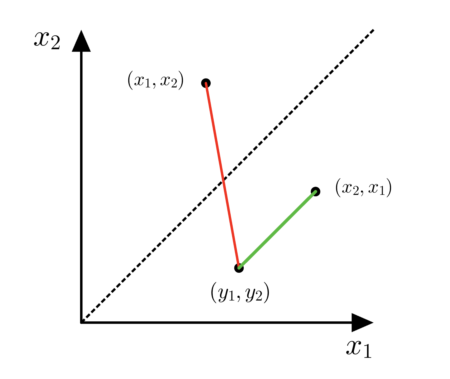
Equivalently, one can “choose a representation” by projecting onto a fundamental domain such as ${x_1 \le x_2}$; doing so selects the smaller of the two distances.
Remark. The expression above is exactly the quadratic Wasserstein distance between the corresponding empirical measures. Indeed, let $\mu^{(n)} = \frac{1}{n}\sum_{i=1}^n \delta_{x_i}$ and $\nu^{(n)} = \frac{1}{n}\sum_{i=1}^n \delta_{y_i}$. The Kantorovich formulation of $W_2$ is
\[W_2^2(\mu^{(n)},\nu^{(n)}) := \min_{\gamma \in \Gamma(\mu^{(n)},\nu^{(n)})} \int |u-v|^2 \, d\gamma(u,v),\]and for equal-weight empirical measures this linear program is equivalent to an optimal assignment problem; in particular, an optimal coupling can be chosen supported on a matching (i.e. a permutation), yielding exactly
\[W_2^2(\mu^{(n)},\nu^{(n)}) = \min_{\sigma \in S_n} \frac{1}{n} \sum_{i=1}^n (x_{\sigma(i)} - y_i)^2 = \|x-y\|_{n,S_n}^2.\]In other words, equipping $\mathbb R^n$ with $|\cdot|_n$ and taking the quotient by $S_n$ induces a natural metric on orbit space by “distance between orbits = infimum distance between representatives,” and this is exactly what the $W_2$ formula computes for uniform empirical measures.
All this is to say, there is a sense this intuition does carry out very naturally to the general case of absolutely continuous measures. For a more precise handling of this quotient approach, see also [Car13, GT19, HMPS23, KLMP13].
Mean Field Neural Networks
In 2018—beyond the discovery of the Neural Tangent Kernel [JGH18] and several related preprints on convergence results [ALS19,DLL+19] (which deserves its own blog post)—a sequence of works developed a mean-field viewpoint for two-layer neural networks [NS17, CB18, MMN18, SS20, RV22] (with several of these appearing first as preprints and later as journal versions). Certainly this is one more anecdotal example in favour of the multiple discovery hypothesis.
Back to the main topic, let us consider input data ${(x^\alpha,y^\alpha)}_{\alpha=1}^m \subset \mathbb{R}^{n_0} \times \mathbb{R}$, and a two-layer network with weights $W \in \mathbb{R}^{n\times n_0}$ and $a \in \mathbb{R}^n$, where $w_i \in \mathbb{R}^{n_0}$ denotes the $i$-th row of $W$, and $\varphi:\mathbb{R}\to\mathbb{R}$ is an activation:
\[f(x;W,a) = \frac{1}{n}\sum_{i=1}^n a_i\,\varphi(\langle w_i, x\rangle).\]The main idea behind mean field networks is that instead of viewing the network as a finite sum, we can write it as an integral against the empirical measure of neuron parameters
\[\rho^{(n)} := \frac{1}{n}\sum_{i=1}^n \delta_{(w_i,a_i)} \quad \text{on } \mathbb{R}^{n_0}\times\mathbb{R},\]so that we can write
\[f(x;\rho^{(n)}) = \int a\,\varphi(\langle w, x\rangle)\, d\rho^{(n)}(w,a) \,,\]and the mean squared error as
\[L(\rho^{(n)}) = \frac{1}{2m} \sum_{\alpha=1}^m \left[ f(x^\alpha; \rho^{(n)}) - y^\alpha \right]^2 \,.\]This terminology comes from interacting particle systems and statistical physics: each neuron $(w_i,a_i)$ is a particle, and the population is summarized by $\rho^{(n)}$. In particular, the representation by $\rho^{(n)}$ reflects the fact that neurons are indistinguishable: permuting the indices $i=1,\dots,n$ does not change the function $f$.
The reason why this mean field view is significant is due to propagation of chaos: in the limit as $n\to\infty$ (and under suitable assumptions), the empirical measure converges $\rho_t^{(n)} \to \rho_{t}$, which is not only the population distribution of all the particles, but also the marginal probability distribution of any single particle!
More precisely,
\[\rho_{t}^{(n)} = \frac{1}{n} \sum_{i=1}^n \delta_{w_{i}, a_{i}} \xrightarrow{} \rho_{t} \xleftarrow{} \mathscr{L}( \{ w_{i}, a_{i} \} ) \,,\]which really implies that instead of tracking a system of $n$ equations, it’s sufficient to track a single equation for $\rho_t$ — a drastic simplification.
This leads to one of the most interesting results from this line of work on mean field networks.
Theorem. (Informal, [NS17, CB18, MMN18, SS20, RV22]) If the neural network is trained via gradient flow, that is
\[\partial_{t} \theta_{t} = - \nabla_{\theta} L(\theta_{t}) \,,\]then the limiting mean field distribution $\rho_{t}$ satisfies the partial differential equation (PDE)
\[\partial_t\rho_t+\operatorname{div}(\rho_t v_t)=0 \,,\]where $\operatorname{div}$ is taken in the parameter variable $(w,a)\in\mathbb R^{n_0}\times\mathbb R$, and the velocity field $v_t(w,a)=(v_t^w(w,a),v_t^a(w,a))$ has components
\[\begin{aligned} v_{t}^w(w,a) &= -\frac{1}{m}\sum_{\alpha=1}^m \bigl(f(x^\alpha;\rho_t)-y^\alpha\bigr)\, a\,\varphi'(\langle w,x^\alpha\rangle)\,x^\alpha \,, \\ v_{t}^a(w,a) &= -\frac{1}{m}\sum_{\alpha=1}^m \bigl(f(x^\alpha;\rho_t)-y^\alpha\bigr)\,\varphi(\langle w,x^\alpha\rangle) \,. \end{aligned}\]Furthermore, this PDE is exactly the Wasserstein gradient flow of $L$ with respect to $W_2$ on the parameter space $\mathbb{R}^{n_0}\times\mathbb{R}$:
\[\partial_{t}\rho_{t} = -\operatorname{grad}_{W_2} L(\rho_{t}) \,.\]This might feel like a surprising result without the context we discussed above, but as we now understand, this is perfectly natural. The quotient map $\pi:\theta\mapsto\rho^{(n)}$ (at least informally) pushes forward the gradient flow dynamics of parameters $\theta_t$ to the induced gradient flow under the quotient geometry, which is Wasserstein gradient flow of $\rho_t$.
As we can see, although this argument is not rigorous, the intuitive connection can allow us to predict the resulting PDE of the neural network training dynamics, without doing any significant derivation at all. This is all because of the clear understanding we have reached with the connection between permutation invariance and Wasserstein geometry.
Concluding Words
In this post, we saw that the geometric understanding of the Wasserstein manifold for probability distributions is not an accident: it’s a rather natural quotient geometry of permutation invariance. The push forward of gradient flow dynamics also naturally yields the Wasserstein gradient flow that we saw in mean field neural networks.
While aesthetically pleasing, I would also like to leave the readers with the question: what can we do with this result? In particular, in the context of mean field neural networks, since the first introduction in 2018, we have made very little progress with these equations and the Wasserstein structure. Hopefully, one of you will be able to use Wasserstein geometry to help us understand neural networks in the future.
References
- [ALS19] Allen-Zhu, Z., Li, Y., & Song, Z. (2019, May). A convergence theory for deep learning via over-parameterization. In International conference on machine learning (pp. 242-252). PMLR.
- [Car13] Cardaliaguet, P. (2013). Notes on mean field games (from P.-L. Lions’ lectures at Collège de France) [Lecture notes]. CEREMADE, Université Paris-Dauphine.
- [CNR24] Chewi, S., Niles-Weed, J., & Rigollet, P. (2024). Statistical optimal transport. arXiv preprint arXiv:2407.18163.
- [CB18] Chizat, L., & Bach, F. (2018). On the global convergence of gradient descent for over-parameterized models using optimal transport. Advances in neural information processing systems, 31.
- [DLL+19] Du, S., Lee, J., Li, H., Wang, L., & Zhai, X. (2019, May). Gradient descent finds global minima of deep neural networks. In International conference on machine learning (pp. 1675-1685). PMLR.
- [GT19] Gangbo, W., & Tudorascu, A. (2019). On differentiability in the Wasserstein space and well-posedness for Hamilton–Jacobi equations. Journal de Mathématiques Pures et Appliquées, 125, 119-174.
- [HMPS23] Harms, P., Michor, P. W., Pennec, X., & Sommer, S. (2023). Geometry of sample spaces. Differential Geometry and its Applications, 90, 102029.
- [JGH18] Jacot, A., Gabriel, F., & Hongler, C. (2018). Neural tangent kernel: Convergence and generalization in neural networks. Advances in neural information processing systems, 31.
- [Lee12] Lee, J. M. (2012). Introduction to Smooth Manifolds (2nd ed.). Springer.
- [KLMP13] Khesin, B., Lenells, J., Misiołek, G., & Preston, S. C. (2013). Geometry of diffeomorphism groups, complete integrability and geometric statistics. Geometric and Functional Analysis, 23(1), 334–366. doi:10.1007/s00039-013-0210-2
- [MMN18] Mei, S., Montanari, A., & Nguyen, P. M. (2018). A mean field view of the landscape of two-layer neural networks. Proceedings of the National Academy of Sciences, 115(33), E7665-E7671.
- [NS17] Nitanda, A., & Suzuki, T. (2017). Stochastic particle gradient descent for infinite ensembles. arXiv preprint arXiv:1712.05438.
- [RV22] Rotskoff, G., & Vanden‐Eijnden, E. (2022). Trainability and accuracy of artificial neural networks: An interacting particle system approach. Communications on Pure and Applied Mathematics, 75(9), 1889-1935.
- [SS20] Sirignano, J., & Spiliopoulos, K. (2020). Mean field analysis of neural networks: A law of large numbers. SIAM Journal on Applied Mathematics, 80(2), 725-752.